CS 499 Homework 1: Basic Parallel Architecture and Communication
- Due: Thursday 2/4/2016 by 11:59 pm
- Approximately 10% of total grade
- Submit to Blackboard in Word or PDF format
- You may work in groups of 2 and submit one assignment per group.
CHANGELOG:
- Thu Feb 4 13:35:04 EST 2016
- Clarifications on problem 5 have been added: only a single algorithm needs to be described, use the same cost model as problem 1 which incorporates the distance between nodes, once a node has the message it can also send it to others, you may assume rows and columns are a power of 2 to simplify the analysis.
- Tue Feb 2 17:46:58 EST 2016
- Submission instructions have been added to the bottom of the HW specification and a submission link has been added to Blackboard.
- Tue Feb 2 13:43:07 EST 2016
- As per a piazza post on the subject, problem 1 now includes a clarification concerning when the startup cost of communication is paid.
Table of Contents
- 1. Problem 1: Store-and-forward Routing (Grama 2.26)
- 2. Problem 2: Shared vs. Distributed Memory Architectures (Grama 2.7, 2.8)
- 3. Problem 3: Task-dependence Graphs (Grama 3.2)
- 4. Problem 4: Parallel Bucket Sort (Grama 3.19, 3.20)
- 5. Problem 5: Parallel One-to-All Broadcast in 2D Torus
- 6. Problem 6: Bring the Heat
- 7. Submission Instructions
1 Problem 1: Store-and-forward Routing (Grama 2.26)
Consider the routing of messages in a parallel computer that uses store-and-forward routing. In such a network, the cost of sending a single message of size \(m\) from \(P_{source}\) to \(P_{destination}\) via a path of length \(d\) is \(t_s + t_w \times d \times m\). An alternate way of sending a message of size m is as follows. The user breaks the message into \(k\) parts each of size \(m/k\), and then sends these \(k\) distinct messages one by one from \(P_{source}\) to \(P_{destination}\). For this new method, derive the expression for time to transfer a message of size \(m\) to a node \(d\) hops away under the following two cases:
- Assume that another message can be sent from \(P_{source}\) as soon as the previous message has reached the next node in the path.
- Assume that another message can be sent from \(P_{source}\) only after the previous message has reached \(P_{destination}\).
For each case, comment on the value of this expression as the value of \(k\) varies between 1 and \(m\). Also, what is the optimal value of \(k\) if \(t_s\) is very large, or if \(t_s = 0\)?
Clarification: To start sending any message, a cost of \(t_s\) must be paid. For example sending \(m=10\) words in its entirety costs \[t_s + t_w \times d \times 10\] Sending the same message broken into two 5-word chunks costs \[(t_s + t_w \times d \times 5) + (t_s + t_w \times d \times 5)\] if the sending does not overlap.
Note: some of the math fonts used above may not display correctly. I have tested the display on Google chrome and seen it work when connected to the network. Notify me if it does not render properly.
1.1 SOLUTION solution
Overlapping messages
In this setting, the source considers the send finished after \(t_s + t_w\times (m/k)\) time as the message will have arrived at the node one hop away (\(h=1\)). The sender can then initiate the next section of the message. This means there will be \(k\) 1-hop sends followed by the final message arriving afterward.
\[ t_{comm} = (t_s + t_w\times (m/k)) \times k + t_w\times (d-1)\times (m/k) \] \[ t_{comm} = k\times t_s + t_w\times m + t_w\times (d-1)\times (m/k) \]
The \(d-1\) is due to the first term accounting for the first hop. With \(k=1\), this reduces to the original model.
Only after reaching destination
The general form is
\[ t_{comm} = (t_s + t_w\times d \times (m/k)) \times k \] \[ t_{comm} = k\times t_s + t_w\times d\times m \]
This is worse than the above form in which message sending can overlap which is seen in the term \(t_w\times d\times m\) here which either lacks the \(d\) or is divided by \(k\) in the setting above.
Comparison for values of \(k\)
As \(k\) increases to \(m\), the left term \(k\times t_s\) grows large in both settings, particularly if \(t_s\) is large. Thus, for large \(t_s\), \(k=1\) is optimal in both settings due to this term.
If \(t_s\) is zero, it makes no difference how many pieces the message is broken into in either model.
2 Problem 2: Shared vs. Distributed Memory Architectures (Grama 2.7, 2.8)
Outline the major differences between a shared memory parallel computer and a distributed memory parallel computer. Discuss the following in your answer.
- Overview the differences in the basic architecture of these two types of machines with respect to memory access.
- Describe how the programming models are different between these two paradigms due to the differences in memory access.
- Report the relative abundance of one architecture versus the other and where they typically appear "in the wild".
- Which architectures scales better as more processors are incorporated. For example, discuss the feasibility of building a 1024 processor computer with 1024 GB of RAM as a distributed memory machine versus as a shared memory machine.
2.1 SOLUTION solution
A: Distributed vs Shared memory
- Distributed memory machine has many processors which do not share memory, each proc owns its own memory, procs connected through some sort of network, explicit communication of sending and receiving is typically required
- Shared memory has many procs all connected to the same memory, can communicate by modifying shared memory, must resolve conflicts according to some scheme
B: Programming Models
- Distributed memory: message passing is typical, explicit communication via send/receive type commands
- Shared memory: threading models are typical, communication through shared variables/memory, requires locking mechanisms to avoid problems
C: Relative Abundance
- Shared memory systems now quite common: most modern CPUs are multicore with same RAM shared
- Distributed less common if explicitly constructed for that purpose though businesses often have server "farms" to get work done, still common in scientific computing, the Internet may be considered one very large distributed memory machine
3 Problem 3: Task-dependence Graphs (Grama 3.2)
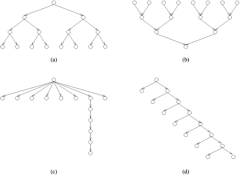
For the task graphs given in Figure 3.42 (below), determine the following:
- Maximum degree of concurrency.
- Critical path length.
- Maximum achievable speedup over one process assuming that an arbitrarily large number of processes is available.
- The minimum number of processes needed to obtain the maximum possible speedup.
- The maximum achievable speedup if the number of processes is limited to 2, 4, and 8.
Assume that each task node takes an equal amount of time to execute.
Figure 3.42. Task-dependency graphs for Problem 3.2.
3.1 SOLUTION solution
A
- 8
- 4
- 15 / 4 = 3.75
- 8
- 8 -> 15/4=3.75, 4 -> 15/5=3, 2 -> 15/8 = 1.875
B
- 8
- 4
- 15 / 4 = 3.75
- 8
- 8 -> 15/4=3.75, 4 -> 15/5=3, 2 -> 15/8 = 1.875
C
- 8
- 7
- 14 / 7 = 2
- 8
- 8 -> 14/7=2, 4 -> 15/8 = 1.875, 2 -> 15/10 = 1.5
D
- 2 with eager scheduling, 8 otherwise
- 8
- 15 / 8 = 1.875
- 2
- 8 -> 15/8 = 1.875, 4 -> 15/8 = 1.875, 2 -> 15/8 = 1.875
4 Problem 4: Parallel Bucket Sort (Grama 3.19, 3.20)
Consider parallelizing the bucket-sort algorithm on a distributed memory computer.
- Input consists of an array
Aofnrandom integers in the range[1...r]. - All
pprocessors on the parallel computer are assumed to have access to the entire arrayAin memory. - The algorithm should compute the array of integers
Bwhere elementB[i]contains the total number of times integeriappeared in input arrayA. - At the end of the algorithm execution, at least one processor must
contain the entire array
Bwhich may involve some communication.
Describe two ways to decompose this problem into a parallel program. Compare these two.
- Describe a decomposition based on partitioning the input data
(i.e., the array
A) and an appropriate mapping onto p processes. Describe briefly how the resulting parallel algorithm would work. - Describe a decomposition based on partitioning the output data
(i.e., the array
B) and an appropriate mapping onto p processes. Describe briefly how the resulting parallel algorithm would work. - Discuss the advantages and disadvantages of these two parallel
formulations. Describe circumstances under which each is
preferred. Such circumstances should consider
pthe number of processorsrthe number of different data possibilities (size ofB)Athe input array andnits size- Potentially also the cost to communicate between the processors
4.1 SOLUTION solution
A Input Decomposition
Divide the input array A into P chunks as evenly as possible: each
processor hold approximately n/P elements of A. Each processor
counts the occurrences of numbers 1..r in its own chunk. After this
calculation is complete, the vectors are summed through
communication/reduction onto a single processor which is the answer
vector B.
B Output Decomposition
Divide the output array B into P chunks as evenly as possible: each
processor hold approximately r/P elements of B. Each processor
must hold a complete copy of the array A which is used to count all
the occurrences of its elements of B. Once done, each processor
communicates its portion of the array B to a lead processor which
concatenates the results to produce the full version of B.
C Advantages/Disadvantages
If A is large (large n) compared to the output of r elements of
B, it may be infeasible for all P processors to store A in
duplicate. This situation lends itself well to the input
decomposition which splits up A into smaller chunks. However this
version involves communication overhead at the end to reduce the
counts down to the final answer.
There are not too many circumstances which would favor the output
decomposition in this formulation of the problem as even if B and
r are very large compared to A and n, the output is still
required to eventually be stored on a single processor. It is likely
to be just as efficient to avoid the communication costs associated
with moving A around and concatenating chunks of B by having a
single processor do the whole computation.
5 Problem 5: Parallel One-to-All Broadcast in 2D Torus
Assume processor 0 has a message that must be sent to all other
processors in a distributed memory parallel computer. Describe an
efficient algorithm to do this in a 2D Torus (wrap-around mesh) with
R rows and C columns.
Account for the following in your answers.
- A processor can send a message to any other processor. Any processor between the source and destination does not receive the message, only forwards it along the path. However, once a processor has actually received the message, it can subsequently be a source and send it to other processors.
- Processors can be indexed with 2D coordinates as in processor (0,2) sends a message to processor (5,4)
- Give rough pseudocode for how this algorithm will look
- Give a cost estimate of this communication in terms of the number or
rows
Rand columnsCin the network. The cost of a single communicate between nodes that are \(d\) hops away is \[t_{single} = t_s + t_w \times m \times d\] You may assume thatRandCare powers of two in your analysis to simplify the expression for the total communication time \(t_{comm}\).
5.1 SOLUTION solution
The torus does not change the nature of broadcast over the mesh. The key idea is to repeatedly double the number of processors which have the broadcast data. This is illustrated in one dimension first on an 8-node line network.
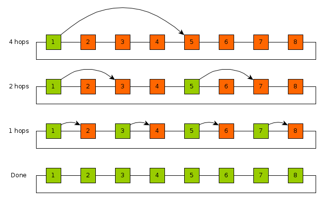
Notably this communication pattern also limits the network contention: each link is used only by one communication at each step.
Assuming the number of columns \(C\) is a power of two and based on the pattern in this diagram the elements of an entire row can be populated in time
\[ t_{row1} = \sum_{i=0}^{\log_2{C}-1} t_s + t_w\times m\times 2^{i} \]
This can be simplified using the identity
\[ \sum_{i=0}^{N-1} 2^i = 2^N -1 \]
which gives the expression
\[ t_{row1} = (\log_2{C}-1)\times t_s + t_w\times m\times (2^{\log_2{C}} -1) \] \[ t_{row1} = (\log_2{C}-1)\times t_s + t_w\times m\times (C-1) \]
The same horizontal process is repeated vertically in each column simultaneously giving \[ t_{cols} = (\log_2{R}-1)\times t_s + t_w\times m\times (R-1) \]
which gives a total cost of \[ t_{comm} = (\log_2{C}-1)\times t_s + t_w\times m\times (C-1) + (\log_2{R}-1)\times t_s + t_w\times m\times (R-1) \] \[ t_{comm} = (\log_2{C}+\log_2{R}-2)\times t_s + t_w\times m\times (C+R-2) \]
Pseudocode:
BroadCast for a torus with R rows and C columns
  Assume R and C are powers of 2
  Message starts on processor 1,1
  for( t=C/2; t>=0; t = t/2 ):
    each proc (1,j) which has message sends it to proc (1,j+t)

  All of row 1 now has messages

  for( t=R/2; t>=0; t = t/2 ):
    each proc (i,j) which has message sends it to proc (i+t,j)

  All processors now have the message
6 Problem 6: Bring the Heat
Consider a simple physical simulation of heat transfer. A rod of material is insulated except at its ends to which are attached two constant sources of heat/cold.
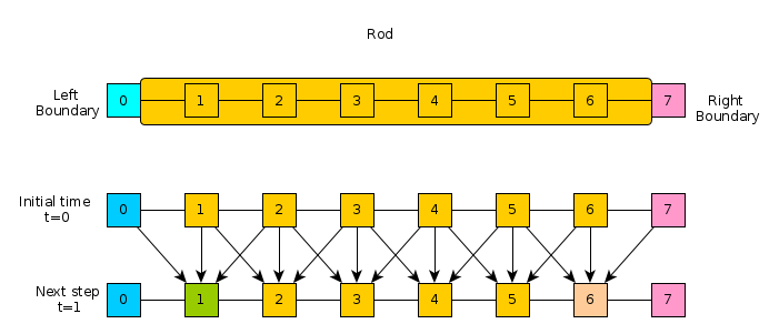
The rod is broken into discrete chunks, sometimes referred to as finite elements, and it is assumed that throughout each element the temperature is uniform. The reservoir elements of heat/cold at the left and right remain at a constant temperature. For the other elements, the temperature is updated at each time step by examining the temperature of its neighbors compared to itself. This dependence is indicated in the lower part of the diagram and the exact update for an element is given in the code below.
The following C code implements a simple version of this simulation.
A row of the matrix H contains the temperature of all elements in
the rod at a time step with the leftmost and rightmost elements
remaining constant. Ultimately, the program computes the entire matrix
H which contains temperatures of all elements at all time steps.
Examine this code carefully.
#include <stdio.h>
#include <stdlib.h>
/* HEAT TRANSFER SIMULATION

   Simple physical simulation of a rod connected at the left and right
   ends to constant temperature heat/cold sources.  All positions on
   the rod are set to an initial temperature.  Each time step, that
   temperature is altered by computing the difference between a cells
   temperature and its left and right neighbors.  A constant k
   (thermal conductivity) adjusts these differences before altering
   the heat at a cell.  Use the following model to compute the heat
   for a position on the rod according to the finite difference
   method.

      left_diff  = H[t][p] - H[t][p-1];
      right_diff = H[t][p] - H[t][p+1];
      delta = -k*( left_diff + right_diff )
      H[t+1][p] = H[t][p] + delta

   Substituting the above, one can get the following

     H[t+1][p] = H[t][p] + k*H[t][p-1] - 2*k*H[t][p] + k*H[t][p+1]

   The matrix H is computed for all time steps and all positions on
   the rod and displayed after running the simulation.  The simulation
   is run for a fixed number of time steps rather than until
   temperatures reach steady state.
*/

int main(int argc, char **argv){
  int max_time = 50;            /* Number of time steps to simulate */
  int width = 20;               /* Number of cells in the rod */
  double initial_temp = 50.0;   /* Initial temp of internal cells  */
  double L_bound_temp = 20.0;   /* Constant temp at Left end of rod */
  double R_bound_temp = 10.0;   /* Constant temp at Right end of rod */
  double k = 0.5;               /* thermal conductivity constant */
  double **H;                   /* 2D array of temps at times/locations  */

  /* Allocate memory  */
  H = malloc(sizeof(double*)*max_time);
  int t,p;
  for(t=0;t<max_time;t++){
    H[t] = malloc(sizeof(double*)*width);
  }

  /* Initialize constant left/right boundary temperatures */
  for(t=0; t<max_time; t++){
    H[t][0] = L_bound_temp;
    H[t][width-1] = R_bound_temp;
  }

  /* Initialize temperatures at time 0 */
  t = 0;
  for(p=1; p<width-1; p++){
    H[t][p] = initial_temp;
  }

  // Simulate the temperature changes for internal cells
  for(t=0; t<max_time-1; t++){
    for(p=1; p<width-1; p++){
      double left_diff  = H[t][p] - H[t][p-1];
      double right_diff = H[t][p] - H[t][p+1];
      double delta = -k*( left_diff + right_diff );
      H[t+1][p] = H[t][p] + delta;
    }
  }

  /* Print results */
  printf("Temperature results for 1D rod\n");
  printf("Time step increases going down rows\n");
  printf("Position on rod changes going accross columns\n");

  /* Column headers */
  printf("%3s| ","");
  for(p=0; p<width; p++){
    printf("%5d ",p);
  }
  printf("\n");
  printf("%3s+-","---");
  for(p=0; p<width; p++){
    printf("------");
  }
  printf("\n");
  /* Row headers and data */
  for(t=0; t<max_time; t++){
    printf("%3d| ",t);
    for(p=0; p<width; p++){
      printf("%5.1f ",H[t][p]);
    }
    printf("\n");
  }

  return 0;
}
Answer the following questions about how to parallelize this code.
- A typical approach to parallelizing programs is to select a loop and split iterations of work between available processors. Describe how one might do this for the heat program. Make sure to indicate any loops for which this approach is not feasible and any which seem more viable to you.
- Describe how you would divide the data for the heat transfer problem among many processors in a distributed memory implementation to facilitate efficient communication and processing. Describe a network architecture that seems to fit this problem well and balances the cost of the network well.
6.1 SOLUTION solution
A Parallelizing loops
The main computation loop is doubly nested iterating over t (time)
in the outer loop and p (position) in the inner loop. Importantly,
there are dependencies between timesteps: row t+1 of the result
matrix H is computed using elements from the previous row t. This
means the task of computing each element are dependent on preceding
tasks of computing rows above it and cannot be done in parallel.
Instead, the best parallelization is on the inner loop. Each position
p is dependent on elements of the preceding row. Thus, all
positions of row H[t+1] can be computed simultaneously provided
access to row H[t].
B Data Distribution
Since it is not possible to parallelize on the rows of the output
matrix, the data should be split along the columns which represent
positions of the rod. Data should be distributed so that adjacent
columns reside on nearby processors. A linear array of processors is
all that is required to keep relevant data close to processors that
need it (a mesh or hypercube can be easily mapped to a linear array).
Each time step t, a processor uses the values it has from the
previous time step in its columns along with a few values transmitted
from adjacent processors to compute part of the row t+1. This keeps
the data needed to compute each partial row fairly local to the
processors that need it which reduces communication costs.
7 Submission Instructions
- Complete the problems in each section labelled Problem
- This is a pair assignment: you may select one partner to work with on this assignment as a group of 2. You may also opt to work alone as a group of 1.
- Only 1 member of your group should submit the HW Writeup on Blackboard
- Make sure the HW Writeup has all group member's information in it:
CS 499 HW 1
Group of 2
Turanga Leela tleela4 G07019321
Philip J Fry pfry99 G00000001
- Do your work in an acceptable electronic format which are
limited to the following
- A Microsoft Word Document (.doc or .docx extension)
- A PDF (portable document format, .pdf)
You may work in other programs (Apple Words, Google Docs, etc.) but make sure you can export/"save as" your work to an acceptable format before submitting it.
- Submit your work to our Blackboard site.
- Log into Blackboard
- Click on CS 499->HW Assignments->HW 1
- Press the button marked "Attach File: Browse My Computer"
- Select your file
- Click submit on Blackboard